This formatting can often be as simple as choosing the right type of data, but it might also involve customizing the format settings until you have the right one. You can remove the dollar sign from currency formatting in Excel 2013 by right-clicking a cell, selecting Format Cells, then clicking the Symbol dropdown menu and choosing the None option. There is often a difference in the way your data appears in cells in Excel 2013 spreadsheets. The number of displayed decimal places can vary depending on the entered amounts so, if you are dealing with monetary values, it’s helpful to keep them consistent by formatting those values as currency. But the default currency formatting in Excel 2013 includes a dollar sign in front of the numbers, which is something that you may not want. Luckily you have control over many aspects of the currency formatting, including whether or not that dollar sign is there. Our guide below will show you the option to adjust if you wish to remove that dollar sign from your currency-formatted cells.
How to Format Money Without the Dollar Sign in Excel 2013
Our guide continues below with additional information on removing a dollar symbol in Excel 2013, including pictures of these steps.
How to Remove the Dollar Sign from Numbers in Excel 2013 (Guide with Pictures)
The steps in this article will assume that the dollar sign is being added to your cell data due to an existing currency formatting setting. If the dollar signs have been entered manually, then adjusting the formatting in this manner may not work.
Step 1: Open your spreadsheet in Excel 2013.
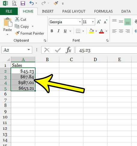
Step 2: Select the cells containing the dollar sign formatting that you want to remove.
You can select an entire column by clicking the column row letter, or an enter row by clicking the column row number.
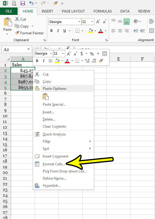
Step 3: Right-click on one of the selected cells, then choose the Format Cells option.
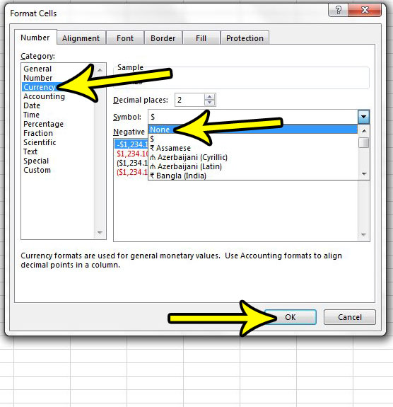
Step 4: Click the Currency option in the column at the left side of the window, click the Symbol dropdown menu and select the None option, then click the OK button at the bottom of the window.
Our tutorial continues below with additional discussion about removing the dollar sign from Excel currency formatting.
More Information on How to Apply Currency Format in Excel 2013
While our steps above discussed editing a format setting in Excel so that you are displaying money without including a dollar symbol, you might be curious about adding the currency formatting in the first place. You can apply Excel currency formatting by selecting the cells that you want to format, then right-clicking on the selection and choosing the Format Cells option. You can then select the Currency option under Category on the left side of the window. You can also choose to use Number formatting, although you are probably at least going to want to set the number of decimal places to 2. Another option that you have for removing dollar symbols is to use the “Find and Replace” tool. You can press Ctrl + F on your keyboard to open it, then click the Replace tab at the top of the Find and Replace window. You can then type a dollar sign into the Find field, then leave the Replace field empty. Then if you click Replace All it should remove all of the dollar symbols that are in the spreadsheet. Have you downloaded a bunch of CSV files that you need to combine into one file, but copying and pasting all of that data will be tedious? Learn about a simple way to quickly combine multiple CSV files using the command prompt.
Additional Reading
He specializes in writing content about iPhones, Android devices, Microsoft Office, and many other popular applications and devices. Read his full bio here.